Conjoint market simulator

To export the conjoint market simulator:

1. Open the Surveys app, go to the Activities page, and open a survey that contains a Choice-Based Conjoint question.
2. On the activity toolbar, click Report.
3. Click Standard Reporting.
4. Click the report that shares the same name as the Choice-Based Conjoint question.
5. Click Export.
6. Follow your web browser's prompts to download and open the conjoint market simulator in Excel.
7. In Excel, enable editing.

   The conjoint market simulator contains four tabs:

   • Simulator
   • Calc
   • Control
   • Util

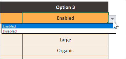
This is the only tab you should interact with and edit. The Simulator tab shows three product profiles alongside a None option.

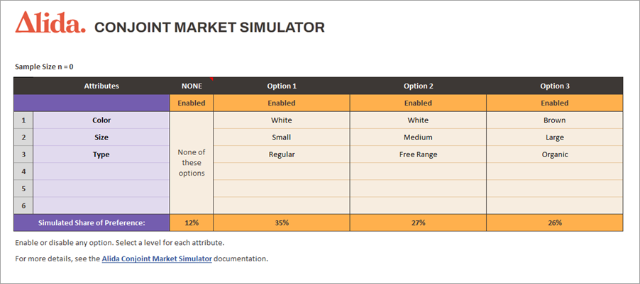
• Enable or disable product profile columns. You can have as many product profile columns enabled or disabled as you like.
• Select the level values from the menus to create different product profiles.

As you make your selections, the conjoint market simulator updates the Simulated Share of Preference value for the product profile.

This tab contains formulas that the conjoint market simulator uses. Do not edit this tab.

This tab contains formulas that the conjoint market simulator uses. Do not edit this tab.

This tab contains raw Choice-Based Conjoint data. Do not edit this tab.

When modeling data, you can choose to apply a single data model to all groups of data in a "one size fits all " approach, or create a custom data model for every single group of data. However, problems arise with both approaches when there are differences in the data groups or how the data is gathered. The "one size fits all" approach may work well for some data groups but not others, particularly if there is variability among the data groups. Similarly, the "one data model per data group" approach works perfectly for one data group, but is less than perfect for other data groups. Hierarchical Bayes (HB) analysis falls somewhere in the middle of these two approaches, which makes it very useful for making predictions.

To picture what HB analysis is doing with your Choice-Based Conjoint data, it might be helpful to think of how HB analysis works in a different context. Imagine you are an ecological researcher who is taking water samples from the same group of ponds every day. Over the course of the year, you collect 365 samples for each pond. The ponds are fairly close together geographically, but still far apart enough for the water quality to be slightly different in each pond. Some days are sunny and warm, while others are rainy and cold. The number of ducks, geese, fish, and plants in each pond vary throughout the year as well. All of these factors could have an indeterminate effect on your samples. Therefore, even if you use the same method and take the water samples at the same time every day, no two samples are obtained in exactly the same way under the same circumstances.

However, some of the water samples may be obtained under similar enough circumstances that you can take known data from the water sample for one pond, and apply it to a water sample from another pond where that same piece of data is unknown and there is a gap. In HB analysis, this is known as borrowing strength. Because each water sample has its own distinct data gaps that other water samples can fill in, the HB analysis will keep repeating this process and borrowing strength until all the data gaps are filled. HB analysis therefore helps make predictions by describing and accounting for the unexplained.

Now let's return to Choice-Based Conjoint data. In HB analysis, an iterative algorithm is used to analyze the existing Choice-Based Conjoint data. As long as the original Choice-Based Conjoint data is high quality and comprehensive enough that the process of borrowing strength can be carried out, the conjoint market simulator can make good predictions. (The exact method used to calculate preference share is called logit share of preference.) What is considered high-quality data for the conjoint market simulator?

• The more responses, the better.
• The more choice sets shown to each participant, the better.
• The more profiles shown to each participant, the better.

The algorithm borrows strength across multiple levels and hundreds of profiles, choice sets, and participants to fill in the gaps and make predictions about preference share. These predictions are an educated best guess and should be taken with a grain of salt, but they can still help you in your decision-making process.